[ad_1]
Amazon QuickSight lately added native assist for comparative (e.g., year-over-year) and cumulative (e.g., year-to-date) interval features which let you simply introduce these calculations in enterprise reporting, development evaluation and time sequence evaluation. This permits authors in QuickSight to implement superior calculations with out having to make use of sophisticated date offsets in calculations to realize such datetime-aware comparisons.
On this submit, we introduce the brand new interval features and their capabilities, and reveal a number of typical use circumstances. We additionally talk about a number of situations to increase the utilization of the interval features, which will probably be helpful in additional superior conditions.
New interval features
Earlier than we reveal use circumstances, let’s go over the brand new interval operate suite and see what new features we now assist. We will divide interval features into two principal teams: comparative (interval over interval) features and cumulative (interval up to now) features.
Comparative (interval over interval) features
You need to use interval over interval features to check measures at completely different time intervals, equivalent to 12 months, quarter, and month. For instance, you’ll be able to compute a year-over-year improve in gross sales, or week-over-week share income modifications.
A typical comparative interval operate has the syntax periodOverPeriodDifference(measure, date, interval, offset), with two optionally available arguments: interval and offset.
You need to use the interval argument within the operate to outline the interval granularity of the calculation. The granularity of YEAR means year-over-year computation, Quarter means quarter-over-quarter, and so forth. If the interval argument is left empty, the calculation modifications primarily based on the interval granularity that’s chosen (within the area effectively) to be displayed within the visible.
You can too use the offset argument to specify what number of intervals aside you need to compute the comparability. As an example, a interval of 1 / 4 with an offset of 2 means evaluating towards the earlier two quarters.
Word that interval and offset should be each specified or each left empty. You possibly can’t specify simply one in all them.
The next desk summarizes the three out there interval over interval features.
| Perform Title | Perform Kind | Description |
| periodOverPeriodDifference | Desk Calculation | Calculates the distinction of a measure over two completely different time intervals as specified by interval granularity and offset. |
| periodOverPeriodLastValue | Desk Calculation | Calculates the final (earlier) worth of a measure from a earlier time interval as specified by interval granularity and offset. |
| periodOverPeriodPercentDifference | Desk Calculation | Calculates the % distinction of a measure over two completely different time intervals as specified by interval granularity and offset. |
Cumulative (interval up to now) features
You need to use interval up to now features to calculate metrics inside a given period-to-date window. There are two principal kinds of cumulative features.
- “OverTime” features, that are desk calculations and return outputs for every row within the visible.
E.g., you should use periodToDateCountOverTime with WEEK granularity to compute a sequence of week-to-date new buyer counts to trace the fluctuation of buyer engagement.
- Aggregation features, which output an aggregated worth for a hard and fast period-to-date time vary.
E.g., periodtoDateSum with YEAR granularity returns a single worth for the entire of the metric from the start of the 12 months to the endDate supplied within the formulation. If left clean, the default endDate takes now(), which is the second when customers load the dashboard.
The next desk summarizes the interval up to now features.
| Perform Title | Perform Kind | Description |
| periodToDateAvgOverTime | Desk Calculation | Calculates the typical of a measure for a given time granularity (as an illustration, 1 / 4) up to a degree in time. |
| periodToDateCountOverTime | Desk Calculation | Calculates the depend of a dimension or measure for a given time granularity (as an illustration, 1 / 4) up to a degree in time. |
| periodToDateMaxOverTime | Desk Calculation | Calculates the utmost of a measure or date for a given time granularity (as an illustration, 1 / 4) up to a degree in time. |
| periodToDateMinOverTime | Desk Calculation | Calculates the minimal of a measure or date for a given time granularity (as an illustration, 1 / 4) up to a degree in time. |
| periodToDateSumOverTime | Desk Calculation | Calculates the sum of a measure for a given time granularity (as an illustration, 1 / 4) up to a degree in time. |
| periodToDateAvg | Aggregation | Averages the set of numbers within the specified measure for a given time granularity (as an illustration, 1 / 4) up to a degree in time. |
| periodToDateCount | Aggregation | Calculates the variety of values in a dimension or measure for a given time granularity (as an illustration, 1 / 4) up to a degree in time, together with duplicates. |
| periodToDateMax | Aggregation | Returns the utmost worth of the desired measure for a given time granularity (as an illustration, 1 / 4) up to a degree in time. |
| periodToDateMedian | Aggregation | Returns the median worth of the desired measure for a given time granularity (as an illustration, 1 / 4) up to a degree in time. |
| periodToDateMin | Aggregation | Returns the minimal worth of the desired measure or date for a given time granularity (as an illustration, 1 / 4) up to a degree in time. |
| periodToDatePercentile | Aggregation | Calculates the percentile primarily based on the precise numbers within the measure for a given time granularity (as an illustration, 1 / 4) up to a degree in time. |
| periodToDatePercentileCont | Aggregation | Calculates the percentile primarily based on a steady distribution of the numbers within the measure for a given time granularity (as an illustration, 1 / 4) up to a degree in time. |
| periodToDateStDev | Aggregation | Calculates the usual deviation of the set of numbers within the specified measure for a given time granularity (as an illustration, 1 / 4) up to a degree in time primarily based on a pattern. |
| periodToDateStDevP | Aggregation | Calculates the inhabitants customary deviation of the set of numbers within the specified measure for a given time granularity (as an illustration, 1 / 4) up to a degree in time primarily based on a pattern. |
| periodtoDateSum | Aggregation | Provides the set of numbers within the specified measure for a given time granularity (as an illustration, 1 / 4) up to a degree in time. |
| periodToDateVar | Aggregation | Calculates the pattern variance of the set of numbers within the specified measure for a given time granularity (as an illustration, 1 / 4) up to a degree in time. |
| periodToDateVarP | Aggregation | Calculates the inhabitants variance of the set of numbers within the specified measure for a given time granularity (as an illustration, 1 / 4) up to a degree in time. |
Use case 1: Utilizing a interval over interval operate to research gross sales development in mounted and dynamic granularity
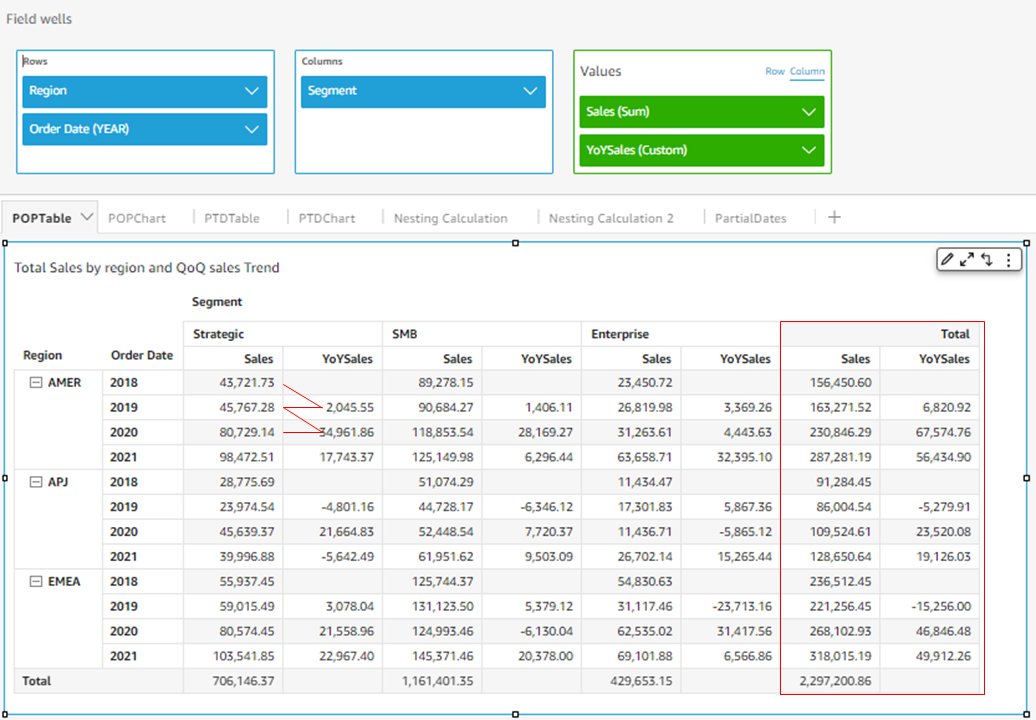
Let’s dive into how interval over interval features can assist typical enterprise and monetary use circumstances. The next instance makes use of periodOverPeriodDifference to calculate YoY gross sales development. As a result of we have now Phase and Area within the visible, the YoY gross sales is calculated for every section and area.
We outline the measure of YoYSales with the next formulation: YoYSales=periodOverPeriodDifference(sum(Gross sales),{Order Date},YEAR,1)
The primary argument, sum(Gross sales), tells the operate to calculate primarily based on this measure. The second argument, Order Date, specifies the date/time column from which Yr data is extracted. The third argument, YEAR, fixes the granularity of this calculation. When this optionally available argument is specified, this measure at all times returns YoY (not QoQ or MoM) regardless of how Order Date is chosen (within the area effectively) to be displayed within the visible. The fourth argument, 1, specifies the offset of the comparability. On this instance, it means we need to examine the gross sales of every order date with the identical date of the earlier 12 months. The measure returns empty for order dates of 2018, as a result of no earlier intervals exist to be in contrast with.
The interval features are working with totals and subtotals. By including the entire for columns into the visible, you’ll be able to see the entire gross sales and whole YoYSales for every area.
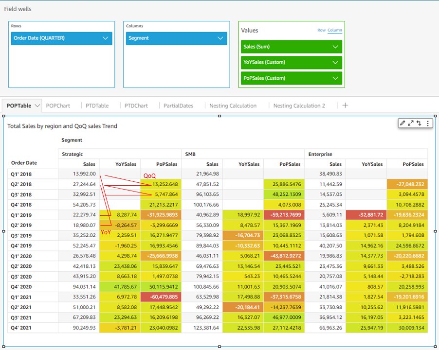
In the event you depart the optionally available argument of interval granularity empty, which means change the formulation to PoPSales=periodOverPeriodDifference(sum(Gross sales),{Order Date})as proven within the following instance, the time interval of the calculation is then decided by the granularity of Order Date displayed on the visible. Within the following instance, Order Date is chosen to show at quarter stage (within the area effectively), so PoPSales dynamically calculates the QoQ gross sales development. Altering Order Date to the month-to-month stage updates the measure to calculate MoM. For PoPSales, solely Q1 2018 returns empty as a result of that’s the one quarter that doesn’t have a earlier quarter to check with.
If we add YoYSales from the earlier instance to this visible, it calculates YoY gross sales development on the quarter stage (compares gross sales of Q1 2019 with Q1 2018). This demonstrates the distinction between a hard and fast granularity and a dynamic granularity of interval over interval features.
The interval over interval features can differentiate between a constructive change (improve) and detrimental change (lower). Due to this fact, once we add the conditional formatting to the visible, it’s very simple to see the monetary efficiency of every interval (inexperienced is sweet, crimson is unhealthy).
Equally, you should use periodOverPeriodPercentDifference to calculate relative gross sales development over time. You possibly can add dimensions into the visible to dive additional into enterprise insights, equivalent to analyzing the breakdown of every enterprise section’s gross sales change by quarter, and their contribution to the entire gross sales improve. We use the formulation PoPSales%=periodOverPeriodPercentDifference(sum(Gross sales),{Order Date}).

Use case 2: Utilizing a interval up to now operate to trace YTD gross sales in desk calculations and aggregations
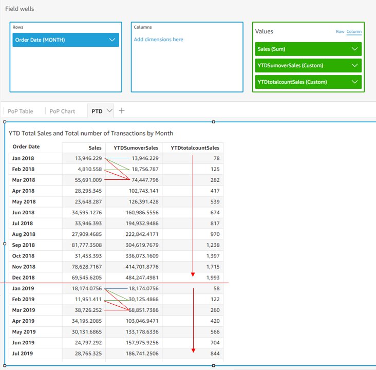
Just like interval over interval features, the interval up to now operate suite gives a fast and straightforward method to calculate year-to-date (YTD) or quarter-to-date (QTD) metrics. Within the following instance, we use the formulation of YTDSumoverSales=periodToDateSumOverTime(sum(Gross sales),{Order Date},YEAR), and YTDtotalcountSales=periodToDateSumOverTime(depend(Gross sales),{Order Date},YEAR) to calculate YTD gross sales and YTD whole variety of transactions.
Opposite to interval over interval features, the third argument of interval up to now features, interval, isn’t optionally available. Due to this fact, the calculation granularity is at all times mounted. On this instance, with the granularity outlined as YEAR, this measure at all times calculates YTD, as a substitute of QTD or MTD. As a result of Order Date is displayed on the month-to-month stage, this calculation outputs the YTD gross sales of every month, and begins over once more in January for the following 12 months. As proven within the outcome desk, YTDSumoverSales of January 2018 is the month-to-month gross sales of January 2018, and YTDSumoverSales of February 2018 is the month-to-month gross sales of January 2018 plus that of February 2018. And YTDSumoverSales of January 2019 goes again to the month-to-month gross sales of January 2019.
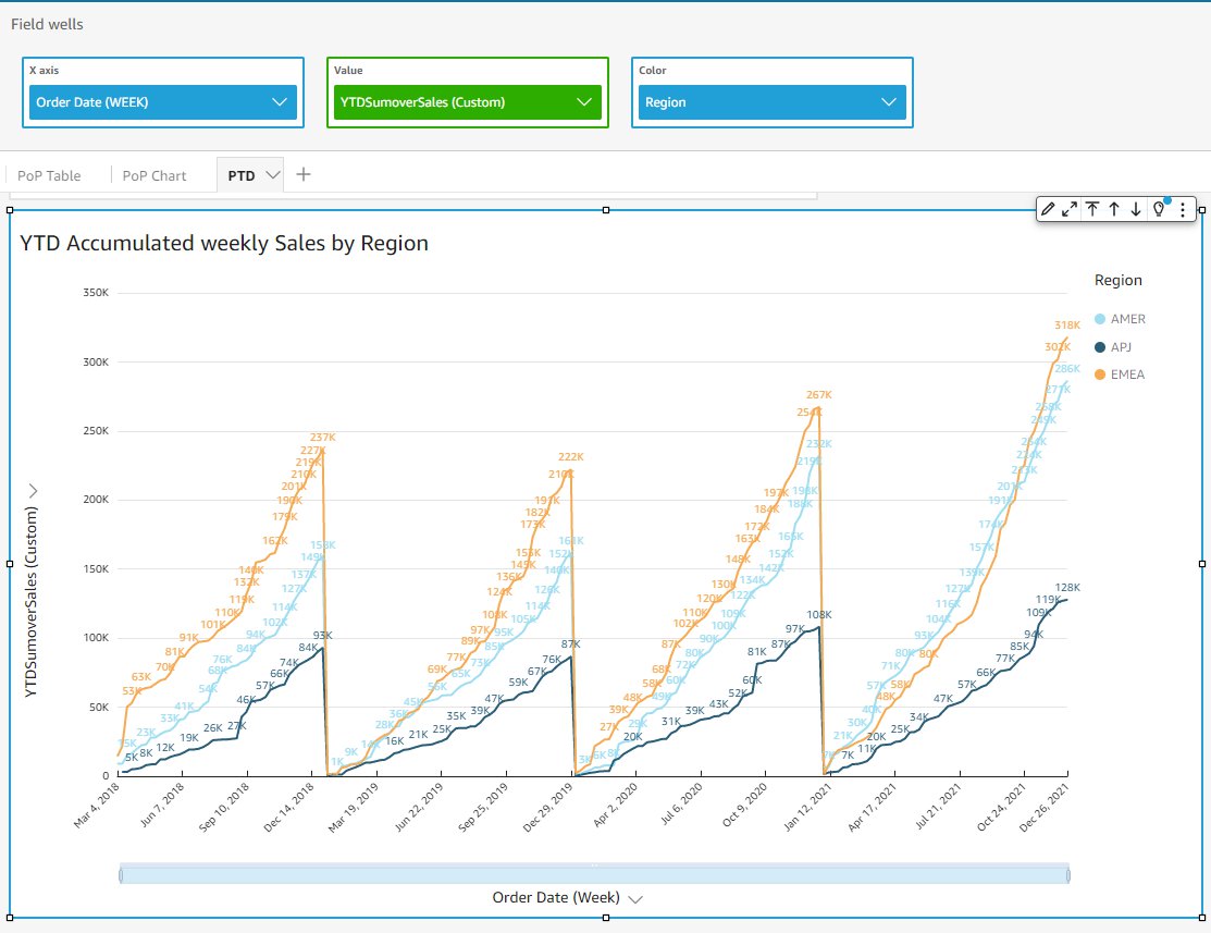
You possibly can additional dive into the small print by populating the calculations in a line chart, and including extra dimensions into the evaluation. The next instance exhibits the YTD weekly gross sales development development for every area alongside the previous 4 years, and uncovers some attention-grabbing gross sales competitors between AMER and EMEA in 12 months 2021.
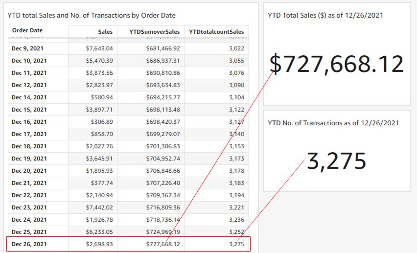
Along with the desk calculations, the aggregation interval features are notably helpful when you must construct KPI charts to judge YTD metrics in a real-time method. Within the following instance, we use the aggregation interval up to now features to construct two KPI charts to trace the YTD whole gross sales, and YTD whole variety of transactions. For the date December 26, 2021, the timestamp outcomes match the corresponding desk calculations for the date of December 26, 2021 within the desk. The next desk summarizes the formulation.
| Formulation | Formulation Kind |
YTDSumoverSales=periodToDateSumOverTime(sum(Gross sales),{Order Date},YEAR) |
Desk Calculation |
YTDtotalcountSales=periodToDateSumOverTime(depend(Gross sales),{Order Date},YEAR) |
Desk Calculation |
YTDSumSales=periodToDateSum(Gross sales,{Order Date},YEAR) |
Aggregation (KPI chart) |
YTDCountSales=periodToDateCount(Gross sales,{Order Date},YEAR) |
Aggregation (KPI chart) |
Superior use case 1: Date/time consciousness with interval features
Interval features will not be solely simpler to outline and skim, they’re additionally date/time-aware, which means the features are calculated primarily based on a date/time-based offset as a substitute of a hard and fast variety of rows. It may possibly remedy two main issues that weren’t attainable to be addressed earlier than.
Interval features can deal with various interval period
If you wish to calculate the every day MoM gross sales improve, you’ll be able to’t use a hard and fast offset on every month as a result of the variety of days of every month are completely different (31 days for January and 28 or 29 days for February).
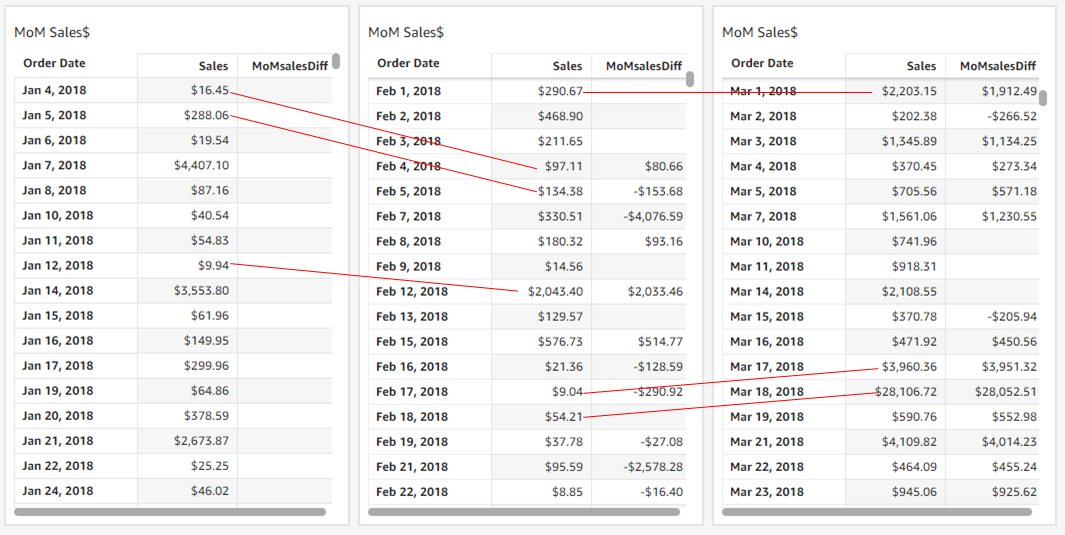
Interval features are calculated primarily based on calendar dates as a substitute of a hard and fast offset. Within the following instance, we use the formulation MoMsalesDiff=periodOverPeriodDifference(sum(Gross sales),{Order Date},MONTH,1). The every day MoM improve is calculated accurately primarily based on the day of the month. The gross sales of the primary day of the month are in contrast with the primary day of the earlier month, and the identical applies to all different days. (Visuals are duplicated for demonstration functions.)
Interval features can deal with sparse (lacking) information factors
Not all datasets can assure an entire set of dates. Within the earlier instance, gross sales information of January 1, 2018, is lacking. Utilizing the workaround primarily based on a hard and fast offset could cause an issue right here as a result of we examine February 1, 2018, with a unique date as a substitute of January 1, 2018. Interval features at all times examine measures by date/time offsets in order that solely desired dates are in contrast. Within the earlier instance, MoMsalesDiff exhibits empty for February 1, 2018, due to the lacking information of January 1, 2018.
Superior use case 2: Nesting interval features with different calculations
Now that we will use interval over interval and interval up to now features to create calculated fields, we will nest these features with different calculations to drive extra superior evaluation.
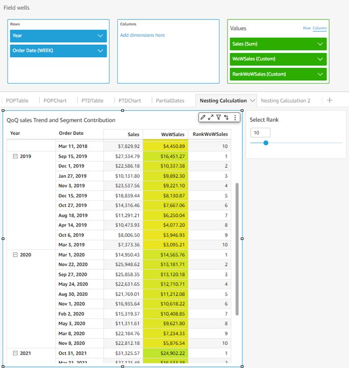
For instance, you might need to know for annually, what are the highest 10 weeks of the 12 months with reference to week-over-week gross sales development. You are able to do this by calculating WoWSales first: WoWSales=periodOverPeriodDifference(sum(Gross sales), {Order Date}, WEEK, 1). Then you definately nest it with the denseRank window operate: RankWoWSales=denseRank([WoWSales DESC],[{YEAR}]). This wouldn’t be attainable utilizing the fixed-row primarily based workaround, which is applied utilizing on-visual calculations as a substitute of calculated fields. Within the following visible, the highest 10 weeks of every 12 months with the very best gross sales development are fetched by a easy filter on RankWoWSales.
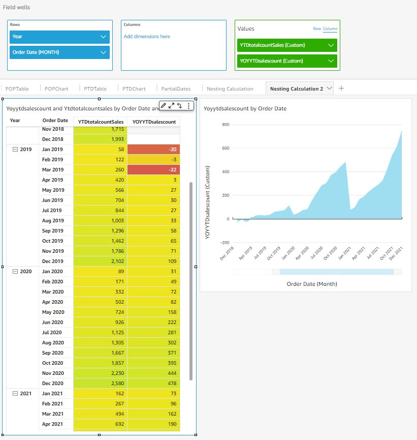
You possibly can even nest the interval features with different interval features to generate attention-grabbing insights. For instance, you’ll be able to calculate a month-to-month YoY development primarily based on the month-to-month YTD variety of transactions. The next formulation demonstrates the potential of nesting a YTD calculated area inside a YoY calculated area:
The ends in the next visible present a YoY development primarily based on a YTD accrued variety of transactions as a substitute of absolutely the month-to-month numbers.
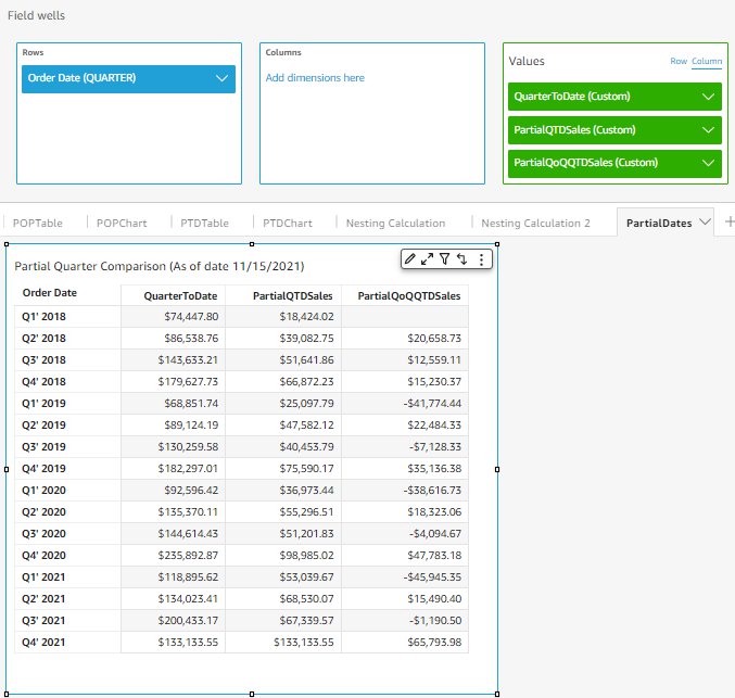
Superior use case 3: Partial interval comparisons
Lastly, we talk about a 3rd superior use case: partial interval comparability. Think about it’s November 15, 2021 (which is the forty sixth day of the final quarter of 2021), and also you need to calculate 4 to check the efficiency of this quarter with previous quarters, however solely utilizing the primary 46 days of every quarter as a substitute of the entire quarter. This requires a calculated area utilizing periodOverPeriodDifference nested with the sumIf() window operate.
The next instance demonstrates utilizing a nested calculated area to handle this use case:
PartialQTDSales computes what number of hours from the start of this quarter to the present date and makes use of sumIf() to calculate the entire gross sales of that interval of every quarter. partialQoQQTDSales then nests the periodOverPeriodDifference operate with PartialQTDSales to seek out the partial QoQ variations. Such a comparability primarily based on a partial interval isn’t possible with out the brand new date/time-aware interval features.
Conclusion
On this weblog, we launched new QuickSight interval features which allow fast and highly effective date/time-based calculations. We reviewed comparative and cumulative interval features (i.e., interval over interval and interval up to now), mentioned two main use circumstances (mounted vs. dynamic granularity and desk calculation vs. aggregation), and prolonged the utilization to 3 superior use circumstances. Interval features at the moment are usually out there in all supported QuickSight Areas.
Trying ahead to your suggestions and tales on the way you apply these calculations for your online business wants.
Concerning the Authors
 Emily Zhu is a Senior Product Supervisor at Amazon QuickSight, AWS’s cloud-native, totally managed SaaS BI service. She leads the event of QuickSight core analytics and calculations functionality. Earlier than becoming a member of AWS, she was working within the Amazon Prime Air drone supply program and the Boeing firm as senior strategist for a number of years. Emily is obsessed with potentials of cloud-based BI options and appears ahead to serving to prospects to advance of their data-driven technique making.
 Rajkumar Haridoss is a Senior Software program Improvement Engineer for AWS QuickSight. He’s the lead engineer on the Question Era group and works on back-end calculations, question planning, and question technology layer in QuickSight. Outdoors of labor, he likes spending high quality time with household and 4-year-old.
[ad_2]


